EpiDEMIC

Short Description

Epifluorescence DEconvolution MICroscopy is a blind deconvolution tool for widefield fluorescence microscopy

Documentation

This plugin contains a blind (i.e. without PSF knowledge) deconvolution method for widefield fluorescence microscopy (a.k.a. epifluorescence) 3D data only. It implements the method described in:

Blind deconvolution of 3D data in wide field fluorescence microscopy, Ferréol Soulez, Loïc Denis, Yves Tourneur, Éric Thiébaut in Proc of International Symposium on Biomedical Imaging, May 2012, Barcelona, Spain.

The code is available here https://github.com/FerreolS/tipi4icy

Tutorial video (in french)

Principle

The blind deconvolution algorithm EpiDEMIC estimates the PSF and the object that minimizes the following equation:

• The first term of this equation is a likelihood cost function that ensures that the model (object convolved by the PSF) is close to the data. It is a weighted least square criterion.  The pixel dependent weights are given by the precision (the inverse variance) of the noise of each pixel.
• The second term is a regularization function that prevents noise amplification. The regularization function used is an hyperbolic approximation the 3D isotropic total variation (TV). This function favors smooth images with sharp edges. The influence of this regularization function has to be tuned by the mean of the so-called hyper-parameter μ.

The plugin is composed of four steps:

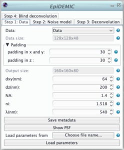
Step 1: Data

• selection of the data and its channel.
• indication of the data size in pixels
• To prevent border artifact the convolution must be performed on a larger size (padding). In theory the padding doubles the size of the data. As this is not possible in practice, the padding size just has to be reasonably large to prevent artifacts.
• As the fast fourier transform algorithm used in the deconvolution is faster for certain dimensions of the images, the output size of the padded image is the most efficient size just larger than the image size plus the padding.
• The lateral size of a pixel (dxy) in nm. Pixel must be square and an error will be raised if the pixel size in x and y retrieved from the metadata differs.
• The distance between to plane (dz).
• The numerical aperture of the objective (NA)
• The refractive index of the immersion medium (ni)
• The emission wavelength (λ)
• All the parameters are retrieved from the data metadata if available. If these metadata have to be corrected, the button “save metadata” saves the parameters given in the plugin as metadata in the icy sequence.

Step 2: Noise model

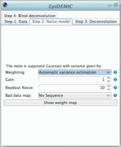The second step defines the noise model used in the likelihood. The noise is supposed to be Gaussian and independently distributed with a variance that varies across pixels. Therefor, the likelihood must be weighted to give more importance to pixels where the noise variance is lower.

This weight map (i.e. inverse variance map)  can set in different manners:

• uniformly distributed noise of variance = 1,
• computed from either inverse variance or variance maps provided by some calibration steps,
• the noise in microscopy is usually a mixture of photon noise and detector noises. If the mean flux is higher than few photons per pixels, this noise can be well modeled by a non stationary Gaussian noise. In this approximation, the computed variance at pixels k is : where γ is the detector gain (number of photons per quantization level) and  is the variance of the readout noise converted in quantization levels. As before deconvolution the object is not known this computed variance is then approximate by:
• After a first deconvolution at step 3, it is possible to have a better estimate of than data. Furthermore, it is also possible to perform a linear regression to automatically estimate detector gain and readout noise.

Some pixels can be dead or saturated. This will destroy the linearity assumed in the convolution model. These pixels must be flagged by zeros in the binary bad data map.

Step 3: Deconvolution

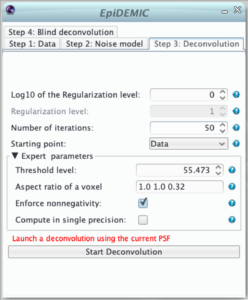Once the data and the noise model are set, it is preferable to perform deconvolution with the aberration free PSF before running the full blind deconvolution algorithm. In this step, it will be possible to tune the regularization level (hyper-parameter μ) and to ensure that no artifact (such as border artifact due to a too narrow padding) will appear.

The main parameters of this panel are  the regularization function parameters that is (for an object f):where:

• μ is the regularization level (hyper-parameter). It ensures the balance between likelihood and regularization. If it is too small the result will be very noisy. If it is too large, details will be smoothed out and the result will be patchy. As it depends of the spatial structure of the objet and the noise level, there is no simple way to choose it and it has to be set by trials and errors. Its behavior is logarithmic and it is more convenient the tune the logarithm of the regularization level
• is the finite difference of the object f at pixel k and along dimension i,
• are the aspect ratio of a voxel.It should be automatically set according to the pixel size.
• ε is a threshold used to smooth the total variation function. The smaller it is the closer to the pristine total variation is the regularization. To help to remove spurious noise this threshold should be similar to the effective quantization level (automatically set as the maximum of the data / 1000).
• By default the object is assumed to be non-negative,

The deconvolution algorithm is iterative. As a consequence, the solution depends on:

• the number of iteration that has to be such has the deconvolved object does not vary from an iteration to another,
• the initial image given as a starting point.

Step 4: Blind deconvolution

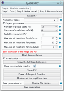
The blind deconvolution algorithm estimates the object and the psf parameters in an alternating fashion. An outer loop is composed of 4 inner optimizations:

1. deconvolution according to the parameters given in panel 3,
2. estimation of the defocus parameters: the refractive index ni (updating the value given in step 1), and the position of the center of the pupil,
3. estimation of the phase of the pupil function,
4. estimation of modulus of the pupil function.

• The number of outer loop must be small to have keep computation time affordable.
• The maximum number of iterations of each inner loop can be set independently. A number of iteration set to 0 will bypass this inner optimization.
• The high is the number of coefficients used to model the phase or the modulus, the higher is the complexity.
• To ensure radially symmetric PSF it is possible to select only even Zernike modes.

Tips

• To perform deconvolution, the data must be correctly sampled according to the Nyquist criterion. This can be checked by examinating the PSF using the show PSF button.
• Due to java limitation, the padded output cannot be larger than 2^31 pixels.
• The memory footprint of the plugin is of the order of 20 times the size of the data. This can be halved by computing in single precision.
• Pixels with values equal to the data type highest value are automatically considered as saturation.
• The regularization level have to be manually tuned. However it should remain constant for all images coming from the same experiments. All the parameters  for a dataset can be saved and conveniently loaded to be used for another dataset.

DEMICS on server

Deconvolution is a memory and computation intensive task and it may not fit in end-users laptop. To process batches of large datasets, both plugins can be used without the Icy GUI on any server with Docker. The docker images of EpiDEMIC can be pulled from docker hub and executed using (for epidemic):

docker run --rm -v FOLDER:/data -e NAME='DATAFILE'   -e XMS=MEMORY ferreol/epidemic'

where:

• FOLDER is the folder were the dataset is,
• DATAFILE is the name of the file and
• MEMORY is the memory size of the JVM (default: 10G).

All the parameters should be stored in an XML file datafile-param.xml in the same folder. This parameter file can be generated easily using the plugin in the Icy GUI. The result will be stored in the file datafile-dec.tif.